Measurements
Measuring impulse responses
The same parameters can be measured in a real room with an exponential sine sweep, a loudspeaker, a measurement microphone and an audio interface:
acoustic-spaces devices                                # pick the interface
acoustic-spaces measure --out hall --device 3 --input 1 2 --loopback 4 \
    --duration 10 --silence 4 --repeats 3 --plot
measure plays the sweep on --output (1 by default), records every --input,
deconvolves the recording and prints the parameters of each microphone. It writes
sweep.wav and its settings, the raw recording.wav, the impulse responses in
ir.wav (one channel per input), measurement.json and, with --plot, a level and
decay plot per input. A --loopback input wired straight to the output removes the
latency of the interface, so arrival times are true times of flight.
Any other player and recorder works too: write the excitation, play it while recording, then deconvolve and analyse:
acoustic-spaces sweep sweep.wav --duration 10 --silence 4 --repeats 3
# ... play sweep.wav and record recording.wav, starting together ...
acoustic-spaces deconvolve recording.wav --sweep sweep.json --out ir.wav
acoustic-spaces analyze ir.wav --plot ir.png --json ir.json
How it works:
The sweep is synchronized (Novak et al., 2015), so harmonic distortion of the loudspeaker lands before the linear response and is cut away. Make the silence after each sweep longer than the reverberation time: the responses are as long as the silence (
--lengthcan shorten them) and no longer, as the next sweep’s distortion lands right after it, and a recording that stops with the excitation lacks the high frequencies of the response beyond it. Only a single sweep recorded for longer gives longer responses, up to the recording’s length less the sweep’s. Repeats are averaged, each doubling lowering the background noise by 3 dB.Deconvolution divides spectra, regularised outside the swept band.
analyzefilters with IEC 61260-1 octave filters (Butterworth, order 3, zero phase), finds where each band sinks into the background noise (Lundeby et al., 1995), cuts it there, subtracts the noise and adds the missing tail (ISO 3382-1, 5.3.4). Digital silence at the end of a file (zero padding, or the shift that removes latency) is not taken for noise: the noise floor is looked for before it. Decay times are left out when a band’s decay does not clear the noise by enough: 20 dB for EDT, 35 dB for T20, 45 dB for T30.A band whose lower edge is at or above half the sample rate holds nothing of its own: all its parameters are left out, and so is the STI. At a sample rate below 11.25 kHz that is the 8 kHz band, from 5.62 kHz up. A band that reaches past half the sample rate (the 4 kHz band at 8 kHz, the 8 kHz band at 16 kHz) is analysed from its part below it, with
--reference-energytaken over the same part. A note says so.Each T20 and T30 comes with its ISO 3382-2 non-linearity ξ (‰) and the decay’s curvature (%), left out with the decay time they check (see Simulation): past 10 ‰ or 10 %, the decay is not straight enough for one decay time to describe it.
G needs the source’s free-field level:
--free-field ff.wav --distance 3uses a measurement of the same source in free field (or with reflections windowed out), and--reference-energy 0.01suits responses made bysimulate.simulate --normalizescales every file of a run by one gain, itsir_gaininparameters.json, and those take 0.01 ×ir_gain².analyzealso prints the STI and STIPA of the room alone and the echo criteria.--lateral 2takes channel 2 as a figure of eight with its null on the source, for LF, LFC and LJ;--ambisonicreads first-order AmbiX (W, Y, Z, X) facing the source, for those and the T30 of X, Y and Z;--binauraltakes two channels as the ears and adds IACC;--stageadds stage support for a response measured 1 m from the source.
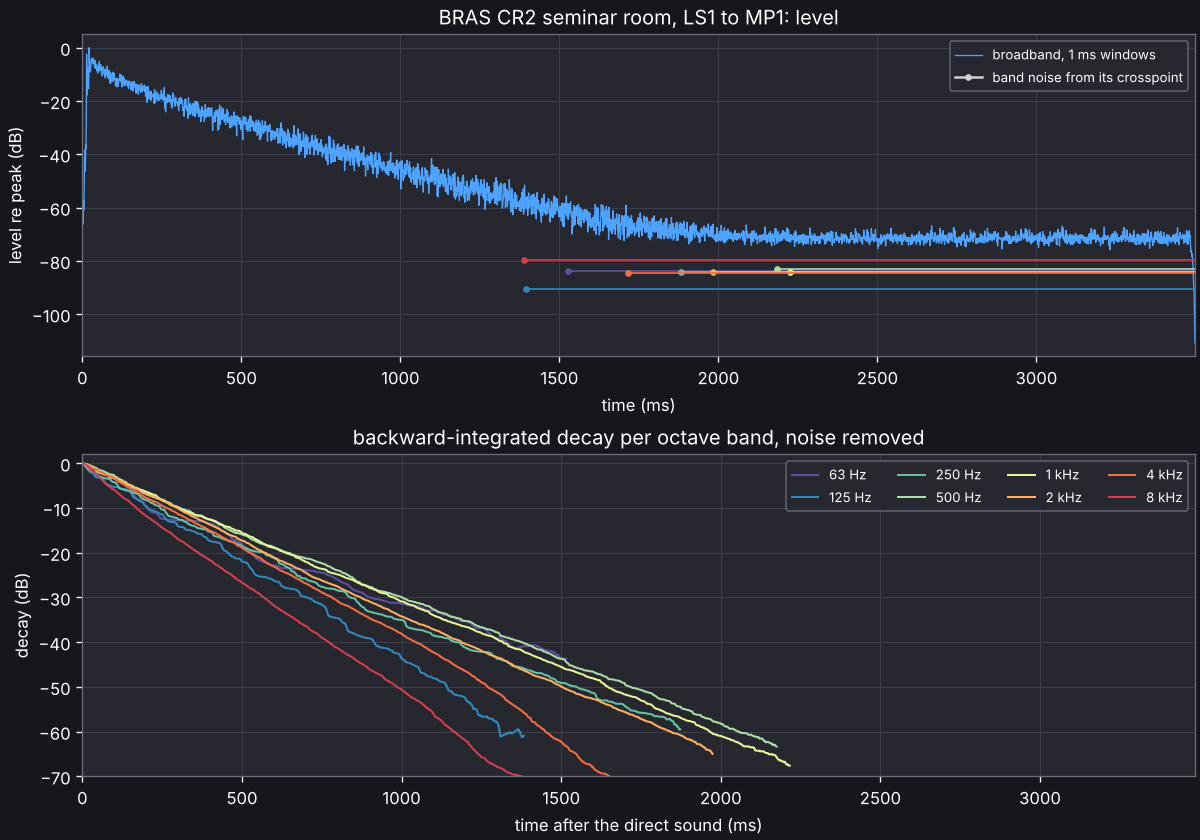
The response above was measured in a seminar room of the BRAS benchmark (Aspöck et al., DOI 10.14279/depositonce-6726.3, CC BY-SA 4.0, which the picture keeps): room CR2, loudspeaker 1 to microphone 1.
From Python:
from acoustic_spaces.measurement import Sweep, deconvolve, measure
from acoustic_spaces.parameters import from_impulse_response

sweep = Sweep(duration_s=10, silence_s=4, repeats=3)
result = measure(sweep, inputs=[1, 2], loopback=4, device=3)
for ir in result.impulse_responses.T:
    print(from_impulse_response(ir, sweep.sample_rate).table())
Comparing with measurements
A model is checked against the room it stands for by comparing its parameters with
those measured there. compare analyses a simulated and a measured impulse response
the same way, each at its own sample rate, and shows band by band how far apart they
are in just noticeable differences (JNDs): 5 % of the measured EDT, 1 dB of C80 and G,
0.05 of D50 and 10 ms of Ts, as ISO 3382-1:2009 gives them (annex A), and by analogy 5 %
of the measured T20 and T30 and 1 dB of C50.
acoustic-spaces simulate hall.yaml --out sim
acoustic-spaces compare sim/talker__seat-a.wav hall/ir.wav --measured-channel 2 \
    --simulated-reference-energy 0.01 --measured-free-field ff.wav --measured-distance 3 \
    --plot compare.png --json compare.json
Its output, for a made-up hall (the numbers show the form, not a result):
simulated: talker__seat-a.wav, channel 1, 48000 Hz, direct sound at 10.1 ms
measured:  ir.wav, channel 2, 48000 Hz, direct sound at 10.0 ms

                  63 Hz  125 Hz  250 Hz  500 Hz   1 kHz   2 kHz   4 kHz   8 kHz
...
T30 (s)   sim     1.533   1.372   1.267   1.111   1.030   1.004   0.899   0.761
          meas        -   1.252   1.214   1.029   1.040   0.959   0.852   0.731
          JNDs        -    +1.9*   +0.9    +1.6*   -0.2    +0.9    +1.1*   +0.8
C50 (dB)  sim      -1.6     2.0    -2.0    -1.9     1.5    -0.1     0.3     1.8
          meas     -1.9     0.7     2.2    -1.2     1.8     0.5     1.3     2.3
          JNDs     +0.2    +1.3*   -4.1*   -0.7    -0.4    -0.6    -1.1*   -0.5
...
JNDs: simulated minus measured, in just noticeable differences; * beyond one
missing:
  T20 at 63 Hz: the measured decay clears the noise by 34 dB, T20 needs 35 dB
  T30 at 63 Hz: the measured decay clears the noise by 34 dB, T30 needs 45 dB

            within 1 JND   mean |JNDs|
EDT (s)           4 of 8           2.0
...
Each JNDs row is the simulated value minus the measured one;
*marks the bands more than one JND apart, where the difference can be heard.The summary gives, per parameter, how many of the compared bands are within one JND, and the mean absolute difference in JNDs from 125 Hz to 4 kHz.
A band where either side has no value shows
-and is listed with the reason, never counted as a difference of zero: a response that decays by less than 20 dB, a decay time whose range does not clear the background noise, G without a reference, or a band above half a response’s sample rate.Each file has its own channel (
--simulated-channel,--measured-channel, 1 by default) and its own reference for G, given as foranalyze:--simulated-reference-energy 0.01suits responses made bysimulate(0.01 ×ir_gain² with--normalize, as above), and the measured side takes--measured-free-fieldwith--measured-distance, or--measured-reference-energy. G is compared only when both sides have one.--filtersand--no-noiseapply to both files.--jsonwrites every value and reason, and--plotoverlays the two decays in each octave band (viz extra).
From Python, compare_impulse_responses does the same, and compare_parameters
compares two sets of parameters already computed:
from acoustic_spaces.audio import read_wav
from acoustic_spaces.compare import compare_impulse_responses

sim, sim_rate = read_wav("sim/talker__seat-a.wav")
meas, meas_rate = read_wav("hall/ir.wav")
comparison = compare_impulse_responses(
    sim[:, 0], sim_rate, meas[:, 1], meas_rate, simulated_reference=0.01
)
print(comparison.table())
t30 = comparison["t30"]
print(t30.difference_jnd, t30.within_jnd, t30.mean_abs_jnd, t30.missing)
compare_parameters also compares LF and LFC (0.05) and IACC_E and IACC_L (0.075,
annex B) where both sets have them, and the directional decay times with the JND of T30.
LJ and stage support have no JND in the standard and are not compared.
Fitting materials to measurements
Absorption from tables seldom matches a room as built. calibrate adjusts the
absorption of the scene’s materials, octave band by octave band, until the simulated
T30, EDT and C80 at each measured source and listener pair come as close as they can to
those measured, in JNDs:
acoustic-spaces calibrate hall.yaml \
    --measured talker seat-a hall/ir_a.wav --measured talker seat-b hall/ir_b.wav \
    -o hall_fitted.yaml --json calibration.json
Its output, for the same made-up hall:
absorption     63 Hz  125 Hz  250 Hz  500 Hz   1 kHz   2 kHz   4 kHz   8 kHz
floor           0.09    0.14    0.23    0.33    0.40    0.46    0.47    0.46
  was           0.13    0.20    0.33    0.46    0.52    0.59    0.59    0.59
  +-            0.36    0.20    0.23    0.08    0.08    0.04    0.08    0.02
...
mean |error|   63 Hz  125 Hz  250 Hz  500 Hz   1 kHz   2 kHz   4 kHz   8 kHz   (JND)
T30 before      5.86    5.84    5.36    5.78    5.32    5.14    5.77    5.06
T30 after       0.04    0.07    0.07    0.11    0.08    0.08    0.06    0.09
...
Each
--measured SOURCE LISTENER FILEis an impulse response measured where the scene has that source and listener: a WAV (its first channel, or--channel), or a report written byanalyze --json.--measured-jsontakes parameters already measured, as{"pairs": {"SOURCE LISTENER": {"t30": [...], "edt": [...]}}}with eight octave values each (null where missing), the format ofvalidation/bras/*/measured.json. A band with no measured value (null, or above half a WAV’s sample rate) is not fitted to, and one that no pair has keeps its absorption.Every material on a surface is fitted (at most 16), or those
--materialsnames;--parameterspicks others to match (T20, C50, D50, Ts, G).The table gives each material’s fitted absorption, what it started from (
was), and+-: its standard error, how far it could move, the other materials following it, before the sum of the squared misses (in JNDs) grows by 1. Where that is a tenth or more, the measurements hardly decide it.-owrites the scene with the fitted absorption (a material given in third octaves keeps its shape within each octave), and--jsonevery number.The materials keep their proportions unless the measurements ask otherwise. Measurements fix the total absorption best. Telling two materials apart needs responses that hear them differently, and surfaces that the sound meets alike (the floor and ceiling of a flat room) trade absorption freely. So the fit may scale every material by a common factor, but moving one by a factor of 2 more than the others costs as much as missing a parameter by one JND. With measurements that cannot tell the materials apart, it is the fit of one factor per band, like fitting the reverberation time with Eyring’s formula, but with the rays of the model itself.
It does not trace the room for every trial. Each round traces it once, counting each ray’s reflections off each material, and the responses for other absorption come from re-weighting those rays (
acoustic_spaces.engine.reweight); the next round traces again at the absorption found, until it moves by less than 0.01 or--rounds(4) run out. Within a round the early reflections keep the phases they were traced with where they add in pressure (up to 125 Hz indoors by default), which the absorption also sets; the next round’s trace has them at the absorption found, and the parameters reported after the fit come from a last trace. A round costs about one simulation of the measured sources at the scene’s rays (--raysoverrides them).It needs stochastic ray tracing in octave bands, without the wave solver.
On the measured rooms of the validation report, fitted to one loudspeaker position from tabulated absorption, the responses at the other position come within about one JND in the seminar room, as with the absorption BRAS fitted with Eyring’s formula, and closer than with it on the decay in the hall and the auditorium. Coupled rooms need responses in each room: fitted to the loudspeaker in one of BRAS’s two coupled rooms, the responses to the one in the other come out 55 JNDs off in EDT.
The fitting example goes through it with made-up measurements of a seminar room whose
back wall was built without the absorbing panels of its design.
From Python:
from acoustic_spaces.calibration import calibrate
from acoustic_spaces.parameters import from_impulse_response

measured = {("talker", "seat-a"): from_impulse_response(ir_a, 48000)}
found = calibrate("hall.yaml", measured)
print(found.table())
found.fitted_scene().to_yaml("hall_fitted.yaml")