Scene files
A scene is a YAML file that names the geometry, the materials, which surface gets
which material, and where the sources and listeners are. See
examples/shoebox/scene.yaml and the schema in
src/acoustic_spaces/scene/model.py.
Frequency-dependent data uses eight octave bands from 63 Hz to 8 kHz, or 24
third-octave bands from 50 Hz to 10 kHz (see Frequency bands).
Geometry
Format |
Read with |
Names used for material assignment |
|---|---|---|
OBJ |
built-in reader |
|
DXF |
ezdxf (3DFACE, MESH, polyface and polygon meshes, closed 3D polylines, block references) |
layer |
glTF / GLB |
material, node and mesh names |
|
STL, PLY, OFF |
trimesh |
file name |
IFC ( |
IfcOpenShell, the |
element name, type name, materials, IFC class |
Collada ( |
built-in reader (triangles, polylists, polygons, nodes and instanced nodes) |
material, geometry name |
SketchUp ( |
openskp, the |
material |
Simple rooms need no CAD file: geometry: {box: [8, 6, 3]} builds a rectangular
room from the origin, and a floor plan is raised to a height (see
examples/lecture_hall/scene.yaml):
geometry:
  floor_plan: [[0, -4], [0, 4], [14, 8], [14, -8]]  # corners, in order, any shape
  height: 6
assignments:
  floor: audience
  ceiling: plaster
  wall_1: wood       # the edge from the first corner to the second
  walls: concrete    # every other wall
OBJ is the recommended exchange format: SketchUp, Rhino, Revit and Blender all
export it with material names. Set geometry.units (m, cm, mm, in, ft)
and, when the file is +y up (Blender’s OBJ default, glTF always), geometry.up_axis: y.
Without units, a DXF file is read in the units its header records ($INSUNITS), an
IFC or Collada file in the units it records, and any other file in metres; a Collada
file’s up axis is the one it records (X_UP, Y_UP or Z_UP). SketchUp’s Collada export
(.dae) is read as it is (see examples/rehearsal_room).
SketchUp files can also be read as they are, with the sketchup extra: openskp reads
them without SketchUp, in metres. That reader is young. Faces are matched to materials
by colour, so give each material its own colour; a face painted differently on its two
sides takes its front’s material; and some files do not read at all (the BRAS
auditorium, for one). An OBJ export from SketchUp is then the way.
Polygons are triangulated, duplicate vertices merged, degenerate faces, copies of a face
(the same corners, turning the same way) and the vertices no face uses dropped, and
faces that meet along an edge are turned to agree with each other (each part of the
model keeps the orientation most of its area has), so a few
faces flipped by the exporter do not spoil the volume or the inside checks. Where a
face’s edge runs past the corners of faces on its other side (a T-junction, which
SketchUp stitches with faces of zero area), the edge is split at those corners, so the
model stays closed; also where two surfaces and a third face meet along the line it runs
past. A stitch whose own corner lies on its edge (within 10 µm) is dropped there, as the
split closes the gap. A model with no faces left is refused, as is one with coordinates
that are not finite numbers or a face that names a vertex the file does not have.
validate then reports surfaces without a material, sources or listeners outside the
room or on a surface (within 1 µm of it, or within 2e-9 of the model’s diagonal where
that is more, twice the least distance at which a ray traced on the CPU meets a face; an
opening, with air on both sides, does not count) and listeners within 1 cm of a source;
it warns about models that are not closed (rays would escape), listeners so close to a
surface or an opening that the late part comes out noisy, and assignments that match
nothing. Errors exit with status 1, and with --strict warnings too. Normals may point
either way:
the room is the space the faces close off, found from the faces themselves (see
Walls, doors and openings), and a panel standing in the
room, with air on both sides, reflects and absorbs on both.
Outdoors
geometry.ground makes a scene outdoors: a flat ground under an open sky, with
buildings (footprints raised to a height), barriers (thin screens along a path),
vegetation (belts of trees, hedges and lone trees, which sound passes through) and the
objects of a model file standing on it. See Outdoor scenes.
geometry:
  ground:
    margin: 30
    zones:                      # parts of the ground with materials of their own
      - {name: road, polygon: [[-40, -4], [60, -4], [60, 4], [-40, 4]]}
  buildings:
    - {name: hall, footprint: [[0, 10], [20, 10], [20, 22], [0, 22]], height: 9}
  barriers:
    - {path: [[30, 6], [30, 20]], height: 3}
  vegetation:
    - {name: hedge, path: [[30, 24], [50, 24]], width: 1.5, height: 2}
The ground can be a terrain, its heights on a grid from a file or given in the scene
(ground.terrain), and the buildings can come from a GeoJSON map
(geometry.buildings_file); see Terrain and
Buildings from a map:
geometry:
  ground:
    terrain: {file: hills.asc}      # or {heights: [[...], ...], spacing: 10}
    map_origin: [552000, 5806000]   # subtracted from the map files' coordinates
  buildings_file: {file: town.geojson, height: height, default_height: 9}
Outdoors, atmosphere sets the wind and the temperature over the ground, which bend
sound down or up, into shadow zones (see
Wind and temperature), their eddies, which blur
the ground dip, scatter sound into shadows and make it flicker (see
Turbulence), and zones, parts of the scene with weather of
their own (see Weather zones):
atmosphere:
  preset: windy                 # neutral, windy, sunny_day or clear_night
  wind: {speed_m_s: 8, direction_deg: 90}   # 8 m/s 10 m up, blowing towards +y
  turbulence: moderate          # weak, moderate or strong, or its structure parameters;
                                # {preset: moderate, height_m: 2}: weaker with height
  zones:                        # polygons in the plan; what they leave out is the scene's
    - {name: lee, polygon: [[120, -60], [300, -60], [300, 60], [120, 60]], wind: {speed_m_s: 1}}
long_term runs an outdoor scene in several weather classes, each holding for a share
of the day, the evening and the night, for the level over a long term and L_den (see
Levels over a long term):
long_term:
  classes:                      # a class takes the scene's weather where it says nothing
    - {name: downwind, share: {day: 0.4, evening: 0.3, night: 0.2}}
    - {name: upwind, wind: {direction_deg: 180}, share: {day: 0.3, evening: 0.2, night: 0.1}}
    - {name: inversion, preset: clear_night, share: {day: 0, evening: 0.3, night: 0.6}}
    - {name: still, preset: neutral, share: {day: 0.3, evening: 0.2, night: 0.1}}
  # periods: [{name: day, hours: 12}, {name: evening, hours: 4, penalty_db: 5},
  #           {name: night, hours: 8, penalty_db: 10}]   # the default, L_den
BIM models (IFC)
IFC files from Revit, ArchiCAD, Vectorworks or any other BIM program are read with the
ifc extra (IfcOpenShell). There are two ways, and
examples/bim_office
shows both:
geometry:
  file: office.ifc
  space: Office        # one room, from its space boundaries; leave out for every element
assignments:
  Plaster on brick: plaster   # an IFC material
  IfcWindow: glass            # every element of a class
  Door: wood                  # one element, by name
With
space, only that room (an IfcSpace, by name, long name or GlobalId) is read: the faces of the room that each element bounds, as BIM programs export them as space boundaries (Revit: export with space boundaries, first or second level). Each face is named after its element; one with no element behind it, an opening to another room, is avirtual boundary. This gives a closed room with one face per surface, which is what the simulation wants. A file without space boundaries gives the space’s own solid, cut into triangles of at most 50 cm, each named after the element behind its middle: windows and doors then have ragged edges, so export boundaries where you can.Without
space, every building element is read as IfcOpenShell builds it: walls, slabs, roofs, windows, doors, stairs and furniture, with their openings cut. Openings, virtual elements and building services (ducts, pipes, lights) are left out. Walls then have both sides and their thickness, and solids that only touch do not share edges, so the model reads as not closed even when no ray escapes (the leak finder tells); the volume and the inside checks are skipped.
Each face’s names, for assignments, are its element’s name, its type’s name, its
materials (a layer set’s name, then each layer’s material) and its IFC class
(IfcWallStandardCase also as IfcWall); the first that an assignment names gives its
material.
Finding leaks
A model that is not closed lets rays escape, and its reverberation comes out too short. The warning counts its open edges; the leak finder shows where the holes are:
acoustic-spaces validate examples/leaky_classroom/scene.yaml --leaks
acoustic-spaces view examples/leaky_classroom/scene.yaml --leaks
leaks: 5000 rays, up to 100 reflections each: 4084 escaped (81.7 %)
  1. 3813 rays (76.3 %) through a gap of about 3.6 m2 (3.00 x 1.20 m) by east_wall
     at (9.00, 3.51, 1.59) m
  2. 271 rays (5.4 %) through a gap of about 0.27 m2 (9.00 x 0.03 m) by ceiling,
     north_wall, west_wall
     at (4.08, 6.99, 3.00) m
It traces rays from the sources (5,000 by default, --rays sets how many), reflecting
them diffusely off every surface whatever its material, so that they reach every corner,
for up to 100 reflections each. Each ray that finds no surface ahead has escaped, and is
put down to the gap it went through: the open edges round a hole, with open edges that
come within 2 % of the model’s size of each other counted as one gap (a ceiling that
stops short of a wall leaves open edges on both). For each gap the report gives the rays
that escaped through it, its area and size (from its open edges, which run round it),
where the rays crossed it and the surfaces next to it, those with the longest open edges
first. In the example the window glass is missing from the east wall and the ceiling
stops 3 cm short of the north wall. view --leaks draws the open edges in red, the
escaping rays from their last reflection to past the hole, and a numbered marker on each
gap; in the editor, View > Show leaks does the same and writes the report to the
messages.
Rays that leave through a surface letting sound through (an opening to the outside, see
Walls, doors and openings) are listed as such, not as a
leak. A closed model keeps every ray; one that loses some all the same has faces that
meet without closing, and the report names them. From Python,
acoustic_spaces.engine.leaks.find_leaks(room) gives the same as a Leaks object, and
acoustic_spaces.viz.plot_leaks draws it.
Materials
Each entry in materials takes coefficients from one of:
preset: <id>: the built-in database (acoustic-spaces materialslists it);file: <csv>: a table of rising centre frequencies in Hz, absorption and optionally scattering, one row each, at any band resolution (the layout the BRAS benchmark uses);file: <library>withentry: <name>: a material of a CATT-Acoustic or ODEON material library (see below);absorption: [...]with eight octave values or 24 third-octave values, which also overrides a preset or file;impedance:a porous ground’s impedance (grass,snow,asphalt… or a flow resistivity;reaction: extendedfor one whose impedance changes with the angle), which gives the absorption and reflects as a ground does (see Ground impedance).
scattering is a number, eight or 24 values, or the id of a built-in scattering entry
(acoustic-spaces materials --kind scattering lists them; theatre_audience, measured
over rows of seated people, rises from 0.3 at 125 Hz to 0.7 from 1 kHz up, and stands
for the rows of an audience area modelled as one raked plane, as CATT-Acoustic and ODEON
models do). Without it a material scatters 0.1 in every band, and a ground with an
impedance nothing (see Ground impedance).
File data with more than one value in some octave (third-octave tables) stays in
third-octave bands; other data is averaged onto octaves. Bands with no data (63 Hz in
most tables) take the nearest band’s value and the material’s source says which.
Coefficients run from 0 to 1: values written in the scene must lie in that range, and a
file’s values outside it (absorption measured in a reverberation room can exceed 1) are
taken as 0 or 1, with a warning that names the material, the file and the bands.
Surfaces get a material through assignments (any geometry name to a material),
by having the same name as a material, or through default_material. Names match
whatever their case (brick_rough names SketchUp’s Brick_Rough), though a name
written the same way wins over one in another case.
uncertainty (Absorption uncertainty on the material’s form in the editor) says
how far a material’s absorption may be off: a standard uncertainty
(distribution: normal, the default) or a tolerance of plus or minus the value
(distribution: uniform), in absorption coefficient units, one value or one per octave
band, with an optional source. A material’s bands are taken as moving together, and
the materials as independent of one another.
materials:
  plaster:
    absorption: [0.02, 0.02, 0.02, 0.03, 0.04, 0.05, 0.05, 0.05]
    uncertainty: {absorption: 0.02, source: lab report}
A built-in material (preset, with no absorption values of its own) that gives no
uncertainty takes simulation.uncertainty.presets, as the built-in database does not
say where its values come from (Built-in materials in the editor’s simulation
settings):
simulation:
  uncertainty:
    presets: tolerance        # tolerance (default), iso_12999_2 or none
tolerance is plus or minus 0.1 in every band; iso_12999_2 is twice the
reproducibility standard deviation that ISO 12999-2:2020 gives for absorption measured
to ISO 354, sigma_R = m alpha + n, as a standard uncertainty: from 250 Hz to 4 kHz the
standard’s octave bands’ (Table 2, for the practical absorption coefficient of
ISO 11654), elsewhere the mean of its third octaves’ (Table 1; the 63 Hz octave from the
63 and 80 Hz rows, the 8 kHz octave, past the table, the 5 kHz row’s); none gives them
none. The standard’s data come from absorbers, and below 100 Hz from outside ISO 354’s
range, so for hard surfaces and the 63 Hz octave it is taken beyond them.
Plus or minus 0.1 is much for a hard surface: the shoebox example’s painted concrete, 0.01 to 0.02, is drawn
anywhere from 0 to 0.12, so that example’s traced T30 at 1 kHz, 1.28 s, lies near the
top of its 95 % interval, 0.74 to 1.49 s. For an absorber ISO 12999-2’s reproducibility
is largest at low frequencies (for alpha = 1, 0.41 at 63 Hz, 0.20 at 125 Hz and 0.040 at
1 kHz), so twice it spreads the lowest bands far. From 500 Hz to 4 kHz it is the same
for every absorption (0.040, and 0.050 at 4 kHz), and a hard surface gets the least in
the lowest bands (for alpha = 0.02, 0.023 at 63 Hz and 0.019 at 125 Hz).
The spread names the materials that took the default (assumed).
acoustic_spaces.engine.uncertainty.material_spread gives the uncertainty this leads to
in each listener’s ISO 3382-1 parameters: the mean, combined standard uncertainty and
95 % coverage interval of many draws, a Monte Carlo propagation as GUM Supplement 1
(JCGM 101:2008) describes. Each draw takes the absorption from its distribution and
re-weights the traced run instead of tracing again, so the run must be simulated with
the materials’ face groups (acoustic_spaces.engine.reweight.groups_of, then
simulate(..., groups=...)), in octave bands, with stochastic ray tracing for the late
part, without the wave solver and with at most 16 materials on its surfaces. A band in
which a material absorbs everything (an absorption of 1, as some absorbers have in some
bands) is not drawn, as no energy is left in it to re-weight; the spread names these
(held). A draw does not go below what the material lets through, which counts as
absorbed. An absorption uncertainty beside a ground’s impedance is left out, with a
warning: the impedance gives the ground’s reflection, which does not follow the
absorption as other surfaces’ do. On a ground with zones, a reflection near a zone’s
edge mixes the grounds on both sides, and a draw takes it as off the ground it meets
alone. To each draw it adds the rays’ random error: the
standard error of the late rays’ batches (simulation.late.batches, 4 or more) times a
deviate of Student’s t with one degree of freedom fewer than the batches, as GUM
Supplement 1 takes a quantity known from that many observations. The budget gives each
input’s standard uncertainty alone (absorption, rays), and the combined one is the
root of the sum of their squares: the rays’ error is added to each draw on its own, so
its variance adds exactly, where the standard deviation of draws that hold it would be
unsteady with few batches. An end of the interval, or a one-sided bound, past what the
parameter can be (a decay time below 0, a D50 above 1) is held at that limit, as the
Analytical Methods Committee recommends near a natural limit (AMC Technical Brief 26A).
The parameters from the late
sound’s directions (LF and the like) have no standard error and take the absorption’s
alone. Not counted: the scattering and the method, and a parameter that some draw leaves
undefined (a decay too slow for the response’s length, say) gets none in that band.
Of the method’s errors, those over edges are listed where a response has paths over
edges (not_counted), each with the largest difference of the level from the exact
solution that Validation
finds in each band, as the band adds its paths in pressure or in energy: over one edge,
over two (second_order), a path reflected on both sides of an edge left out
(one_side), and where a path reaches an edge’s end (a solid block’s corners; a thin
screen’s edges fade out past their ends). Where the solver for whole
rows carries a row’s sound, its
own largest difference from the wave
calculation is
listed in those bands (whole rows) and the edges’ in the others. That sound stays as
it was traced in every draw, though it depends on the absorption of a ground without an
impedance. The method’s errors are not drawn, as they are measured for whole levels in a
few geometries, not for each path.
In the lowest bands, where the early paths add in pressure, a reflection’s phase
follows its face’s admittance, which is fitted to the absorption; the draws take it
between fits at nine absorptions of each material over their range rather than a fit
of their own: in the shoebox example G within 0.17 dB and C80 within 0.20 dB of a fit
for each draw at 63 Hz, where a fit of its own moves them by as much for a change of
0.001 in the absorption (0.18 and 0.23 dB in one of the draws furthest off).
acoustic-spaces simulate does this itself when a material on the surfaces has an
uncertainty, its own or a built-in material’s: it prints the largest combined standard
uncertainty in JNDs from 125 Hz to 4 kHz, with its budget, 95 % interval, one-sided
bounds and the errors over edges, and parameters.json holds them all (uncertainty). With settings that cannot re-weight
(third-octave bands, say) it leaves the spread out and says what the spread needs, as a
warning when a material gives an uncertainty of its own; so does the editor, in its
messages. The editor shows each run’s results at once, draws the spread
after them and gives it in the results table’s tips. The draws add to a run: in the
concert hall example (five built-in materials, six responses) 400 draws take 21 s in
four worker processes (below; 72 s in the run’s own process) after a 12 s run on four
cores, about half of their work the lowest bands’ paths added in pressure for each draw;
presets: none leaves the built-in materials out.
acoustic-spaces simulate and the editor work the draws out in worker processes, as
many as the run has threads (simulation.performance.threads, --threads) and the
cores it may use, with the same results as in the run’s own process and the same
messages. Each process takes a run of one response’s draws at a time and holds that
response, as traced and as a draw re-weights it, what the run’s draws share (up to 128
MiB of the coherent bands’ delay phases and band grids) and its own interpreter, some 80
MiB; the processes take at most half of the computer’s memory (or of its container’s
limit) together, so fewer of them for large responses. There is one process for each
100 draws of all the responses together at most, so a spread of fewer than 200 draws in
all stays in the run’s own process, as does every spread with --threads 1. The
admittances the draws take in the lowest bands are fitted before the draws, each once.
The processes inherit the run’s environment and the cores it may use and set nothing of
the linear algebra’s threads: a draw’s products are added in a fixed order, and the
library’s solvers (the admittances’ fits) run in them as in the run’s own process. The
results come out the same to the last bit, except on an Intel Mac, where Apple’s
Accelerate rounds a sum by where its numbers lie in memory and the admittances’ fits may
differ in their last digits as they may from one fit to the next in one process. In
Python, material_spread and with_spread take workers (1, the default, for none; 0
for every core). The draws stay in the calling process in a daemonic process (a
multiprocessing.Pool’s). The processes are started by spawning, which imports the main
module again in each, so a script that gives workers must do so under
if __name__ == "__main__":, or the call ends with an error.
simulation.uncertainty.draws is the number of draws: 400 unless the scene says
otherwise, 0 for no spread (--spread-draws on the command line, Draws in the
editor’s simulation settings). For a normal spread, 400 draws leave the standard
uncertainty good to about 7 % and each end of the 95 % interval to about a quarter of the
standard uncertainty (twice their own standard deviation). With draws: adaptive the
draws go on as the adaptive procedure of GUM Supplement 1 has them (JCGM 101:2008, 7.9):
batch after batch until, for every result in every band of every response, twice the
standard deviation of the mean, of the standard uncertainty and of each end of the
interval (and of each one-sided bound, below) is within the numerical tolerance of the
standard uncertainty, half a unit of its first digit. A batch is 100 draws, not the Supplement’s 10 000 (a number it calls
arbitrary), as each draw re-weights the whole run; the test is first made after ten
batches, as two this small can pass by chance; and the draws stop at 20 000, the
Supplement’s own first test. stable in parameters.json says whether the test was met
(null for a number of draws given beforehand, which is not tested). The test asks for
many more draws than the default: from 9 000 to 14 500 in runs of the shoebox example.
For a limit on one side, the spread gives each result’s one-sided bounds from the same
draws (at_least and at_most in parameters.json): the value the result is at least
with a probability of 95 %, and the one it is at most with that probability; for a normal
spread, the mean less and plus 1.645 standard uncertainties, where the 95 % interval’s
ends lie 1.96 away and leave 2.5 % out on each side. simulation.uncertainty.one_sided
gives another probability between 0.5 and 1, 0.9 say (--one-sided on the command line,
One-sided bounds in the editor’s simulation settings).
The same draws give the spread of each listener’s levels and speech results
(uncertainty.levels in parameters.json, with the same parts): the sound pressure
level per octave band and A-weighted, the STI, the STIPA, U50 and, outdoors, the level
relative to free field. Each draw finds them for the source’s sound power and the
scene’s background noise, and their rays’ error comes from the same batches. A band’s
level is its G and the source’s power, so its spread is G’s; in a band whose G some draw
leaves undefined, the level is that of the energy the response holds and has a spread of
its own. simulate prints the
A-weighted level’s with the level it is at most and the STI’s with the STI it is at
least, and the editor’s tips give the level’s in each band. A coverage map gets the
uncertainty of its values by tracing it again for each material (see
Coverage maps); a listener’s insertion loss and
long-term levels have no spread.
Material libraries of CATT-Acoustic and ODEON
Materials kept for CATT-Acoustic or ODEON can be used as they are. file names the
library and entry the material in it: its name (in any case), or for ODEON its
number or description.
materials:
  carpet:
    file: catt_materials.geo   # CATT-Acoustic: ABS lines, in a geometry or library file
    entry: carpet
  ceiling_tiles:
    file: odeon_materials.li8  # ODEON: Material.Li8 or a library of the same layout
    entry: 1001
    scattering: 0.1
CATT-Acoustic writes
ABS name = <a125 a250 a500 a1k a2k a4k> L <s125 ... s4k> {r g b}: absorption and scattering in percent from 125 Hz to 4 kHz, 8 and 16 kHz optional (<a125 ... a4k : a8k a16k>),;before a comment;ABS1gives them as fractions from 0 to 1.ABS name = othergives a material another’s values. Any file with such lines will do (a.geofile with its geometry, or a library). Scattering that CATT estimates itself (L <estimate(...)>) is not read, so givescattering.ODEON’s library has each material on two lines, its number and description, then eight absorption coefficients from 63 Hz to 8 kHz (six, from 125 Hz to 4 kHz, in older libraries). Where the description has ODEON’s
{Product name*=...}and{Category=...}fields, as in its ownMaterial.Li8, the product name is the material’s name, andmaterials --filelists the materials by category. Materials made with ODEON’s Material calculator are read by their octave values, which ODEON simulates with; their third-octave values are not read. ODEON gives scattering to surfaces, so give it withscattering(0.1 otherwise).
The 63 Hz band takes the 125 Hz value where a library has none, 8 kHz the 4 kHz value,
and 16 kHz is left out. acoustic-spaces materials --file <library> lists a library’s
materials, with words to search for as in the built-in database, and in the editor
Edit > Add material from a library picks one. The material_libraries example
takes its carpet and walls from a CATT file and its ceiling from an ODEON one.
Four rooms of the BRAS benchmark, converted from its SketchUp models, are in
validation/bras
as scenes with their surface data and measurements (the coupled rooms twice, with the
door between them at two angles).
Walls, doors and openings
A model can hold several rooms. Sound passes between them through surfaces whose
material lets some through: transmission, the share that passes (1 for an opening),
or transmission_loss, the sound reduction index R in dB (the share is 10^(-R/10)),
one value or one per band.
materials:
  partition:                 # 12 cm of brick
    absorption: [0.02, 0.02, 0.03, 0.04, 0.05, 0.07, 0.07, 0.07]
    transmission_loss: [30, 35, 40, 46, 52, 57, 60, 60]
  door:
    absorption: [0.1, 0.1, 0.1, 0.1, 0.1, 0.1, 0.1, 0.1]
    transmission_loss: 25
  doorway: {transmission: 1}  # an opening: all of it passes
assignments:
  wall_between: partition
  door_leaf: door
  door_hole: doorway
What passes through counts as absorbed on the side it comes from, so the absorption must be at least the transmission in every band. A material without absorption values, preset or file absorbs what it lets through: an opening absorbs 1. What a surface lets out of the rooms goes into no room and does not come back in through another: the late part’s rays and the rain of their reflections stop there.
The rooms are found from the faces: every space the faces close off on all sides is one, whichever way the normals point. The space inside a thick wall or a column, with rooms all round it, is solid, as is the inside of a closed shell standing on the floor or in a corner, its faces lying on the room’s. Such a solid holds air when a source or listener stands in it and a surface that lets sound through joins it to a room (a booth with glass walls), and so does any space it opens into that way; a source or listener inside any other solid is reported as inside a closed solid, and
simulaterefuses to run. When none stands in the model’s rooms (walls drawn as a closed shell inside another), the spaces they stand in are the rooms. A material withtransmission: 0lets nothing through. The faces between two rooms have a room on both sides and reflect and absorb in both.inspectlists the rooms (“closed, 2 rooms of 48.00, 72.00 m3”), the editor too, and the volume is theirs together. When the sources and listeners stand in air that the model’s rooms do not include (walls drawn as a closed shell inside another),inspectalso gives that “air volume”, the one its reverberation times use.Early reflections pass through those surfaces, keeping the share that passes at each; through openings they pass unchanged. A reflected path through more than two partitions is left to the late part, which with the stochastic method counts it (the statistical method takes what the early paths carry out of its own energy, so there the early part keeps any it finds). The rays of the late part that hit a partition go on as two: the reflection, and a copy behind it with the share that passes, so even a 60 dB wall has rays behind it. Each room’s rays are thinned and split for the level that room is expected to reach (from the rooms’ power balance in a diffuse field), so a quiet room behind a wall is traced as finely as the loud one. The detector spheres are sized for the volume of all the rooms, which the rays spread over: sized from the volume of a side room behind a 10 or 40 dB wall, they gave the same G, C80 and T30 there with half as much again spread between seeds. Sound goes straight through, in the direction it came.
Coverage maps cover the audience areas of every room and find at each point what a listener there would. The statistical late method follows coupled-room theory: each room’s diffuse field decays as the energy the rooms exchange through the faces between them has it, with Eyring’s absorption in each, so a room behind a partition holds less and a dry room opening into a live one decays in two slopes; the early paths end at the mixing time of the listener’s room. The statistical reverberation times of
inspectcount each face between two rooms on both its sides, as for one room.For diffraction an opening is a hole: the edges of a doorway are the free edges of the wall round it, and sound bends round them into the next room. Diffraction through a wall is left out, as it is far weaker than what passes straight through.
The wave solver lets its air flow through openings; it does not model walls that let part of the sound through, and says so. Particles in animations pass through openings, and through partitions as often as the sound does.
A listener in a room that no surface joins to the source’s room is warned about.
In the editor, a material’s Lets through chooses nothing, part of the sound (the sound reduction index per band in the table) or everything (an opening).
The tests check the level behind a 30 and a 50 dB partition between two rooms against diffuse-field theory (within 0.3 dB), two rooms joined by an opening the size of the wall against one room of both their sizes, and the double-sloped decay of a dry room opening into a live one against the two-room model (within 1 dB down to -40 dB). The statistical method follows that model in both rooms, and maps over both rooms match listeners at their points. In four rooms in a row, the fourth room’s response is the same whether the early part follows reflections to order 3 or not at all, and ray tracing finds the same early paths as image sources in every room.
The apartment example has a wall and a door, closed or open, between the living room
and the bedroom of a flat.
Audience seating
Sound that reaches a listener low over rows of seats loses much more than the seats’
absorption says, as it passes heads and seat backs on the way. Mark the seating’s
material with audience: true (in the editor, Audience seating):
materials:
  seats: {preset: audience_wooden_chairs_1_m2, scattering: theatre_audience, audience: true}
The attenuation is the fit of Jurkiewicz, Rummler, Green, Wulfrank and Kahle (“Impact of grazing incidence attenuation on early reflection design”, Proc. IOA 47 Pt. 1, 2025) to scale-model measurements over a seated audience: sound arriving at an elevation φ above the audience, having run d metres over it, keeps min(1, (3.40 sin²φ + 2.17 sin φ + 0.02)^((d - 1)/10)) of its energy. That is 17 dB less at grazing incidence after 11 m, 0.6 dB per metre at 5°, and nothing lost from 17.8° up.
It applies to the last leg of every early path (the direct sound, reflections and diffracted sound) to listeners and map points up to 2 m above audience surfaces: φ is the leg’s elevation above the surface under the listener, and d how far the leg runs over audience surfaces no more than 2 m higher than the listener’s ears are above theirs, so the stalls do not shade a balcony seat.
Only in the 500 Hz to 2 kHz octaves (third octaves from 400 Hz to 2.5 kHz), the bands of the fit, where it hardly changed with frequency. The seat dip lower down depends on the seats themselves, and the fit has no data higher up. The late part is left as it is, and the statistical method does not make up what the seats take from the early paths. Leaving out the leg from the source to the first reflection, as the fit does, errs on the side of too little attenuation.
In a flat lecture hall with the talker at 1.6 m, it takes 10 dB off the direct sound at the back row in those bands and 1.3 dB off C50 there.
The town_hall_pa example marks its seats as audience.
Sources and directivity
A source has a position, an orientation (yaw, pitch and roll in degrees; all zero
faces +x with +z up), a sound power level (level_db, dB re 1 pW) and a
directivity:
sources:
  - name: talker
    position: [2.0, 3.0, 1.5]
    orientation: {yaw: 30}
    directivity: cardioid   # or omni, subcardioid, supercardioid, hypercardioid, figure8
  - name: monitor
    position: [0.7, 1.3, 1.2]
    directivity:            # a pattern, or the a of a + (1 - a) cos(theta), per octave band
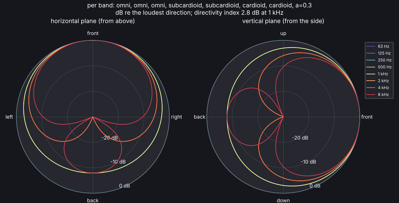
      pattern: [omni, omni, omni, subcardioid, subcardioid, cardioid, cardioid, 0.3]
  - name: loudspeaker
    position: [0.7, 3.3, 1.2]
    directivity: {file: speaker.sofa}   # measured data: SOFA or CSV
A directivity says where the sound power goes, not how much: its weights average 1 over the sphere in every band. It shapes the direct sound, each early path (by the direction it leaves the source in), the rays of the late part and the particles of
animate.SOFA files follow the AES69
FreeFieldDirectivityTFconvention (spectra measured by microphones around the source, as published for loudspeakers and instruments), or hold impulse responses inData.IR. Directions are the microphones’ positions as the source sees them (SourceViewandSourceUp).measurement: 3picks one measurement, for example one note of an instrument; by default all are averaged. Reading SOFA files needs thesofaextra (h5py).A CSV table has the header
azimuth, elevationfollowed by frequencies in Hz, then one row per direction with levels in dB (any reference; only differences matter). Azimuth turns from the front towards the source’s left and elevation is positive upwards, in degrees. Any set of directions works. Bands are averaged into octaves, and octaves with no data copy the nearest one; in third-octave runs each octave’s pattern holds for its thirds. From Python,acoustic_spaces.directivity.write_directivity_csv(path, balloon)writes a directivity (aBalloon) as such a table, its octave bands on its grid.The directions of a SOFA or CSV file are interpolated onto a 5 degree grid, each of its points from the four directions nearest to it, or from all of them where the file has fewer. Where several are equally near and not all of them are among the four, the point takes the nearer ones alone, or all of them if none is nearer. A direction given more than once (a table’s -180 and 180 degrees of azimuth, its rows straight up and down) counts once, with the mean of its energies.
CLF (Common Loudspeaker Format) files are not read: their specification is not public. Convert them to SOFA or CSV.
acoustic-spaces directivity speaker.sofa --plot polar.png prints the directivity
index and front-to-back ratio per octave band and draws the polar patterns;
acoustic-spaces inspect lists every source’s directivity index.
A coherent array, such as a column loudspeaker or a line array, is a source whose directivity is the sum of its elements’ sound with its phase:
sources:
  - name: column
    position: [0.5, 3.0, 2.0]
    directivity:
      array:
        element: cardioid    # each element's pattern, along its aim (default omni)
        count: 8             # a straight column along the up axis, centred...
        spacing_m: 0.15      # ...and this far apart
        steer_deg: -8        # delays that tilt the beam 8 degrees down
  - name: flown
    position: [6.0, 3.0, 6.0]
    directivity: {file: line_array.yaml}   # the same fields in a YAML file
# line_array.yaml: elements one by one, in the source's frame (x forward, y left, z up)
element: {file: cabinet.sofa}   # or a pattern, as for a source
elements:
  - {position: [0, 0, 0.0], orientation: {pitch: 0}}
  - {position: [0, 0, -0.35], orientation: {pitch: -3}, gain_db: -1, delay_ms: 0.05}
  - {position: [-0.02, 0, -0.70], orientation: {pitch: -7}, gain_db: -2}
  - {position: [0, 0, -1.05], invert: true}   # polarity inverted
The elements’ pressures add up with their path differences, their feeds’ gains, delays and polarities, the steering, and each element’s pattern along its aim (first-order patterns with their sign, measured ones by magnitude). The energy is the exact mean over each third-octave band, on a grid of 1 to 5 degrees fine enough for the beam, and with the room’s speed of sound. A column of 8 takes about a second.
The result is the array’s far-field pattern, a balloon like a measured one, so the source stays one point: right beyond about the array’s length squared over the wavelength, L² f / c (16 m for a 2 m array at 1.4 kHz). Closer to a long array, its sound spreads as a line’s and its beam has not formed yet. The room’s warnings name every listener nearer to an array than that distance at 1 kHz:
validate,inspect,simulateandmapprint them, and the editor lists them under Properties when the scene itself is selected. Higher up the far field starts farther still:array length
far field from, at 1 kHz
at 4 kHz
0.5 m
0.7 m
2.9 m
1 m
2.9 m
11.7 m
2 m
11.7 m
46.6 m
near_field: true(next toarrayorfile) adds up the elements’ sound one by one instead, each from where it is, with its own distance, direction, feed and pattern, wherever an early path leaves the array: the direct sound and the reflections (from the image of the listener the path unfolds to), the ground’s reflection and refracted rays outdoors, and the sound that reaches an edge or a crest before it bends round it. It is exact over each band as the pattern is, becomes the pattern far away, and the warnings leave the array out. The late reverberation keeps the pattern, which carries the same power. In the editor it is “Add up the array’s elements one by one” under the source’s directivity.directivity: {file: line_array.yaml, near_field: true}
A 3.75 m column loses about 3 dB per doubling of the distance on axis within its far field’s start, as a line does, and 6 dB beyond it, as a point does.
As for any source,
level_dbis the array’s sound power in all; the pattern only says where it goes. A single element’s array has the element’s own pattern.The tests check a column against the analytic sums of a line array (the directivity index within 0.05 dB in every band, the vertical pattern within 0.3 dB), steering against delays given element by element, a dipole made of two elements in opposite polarity, and splayed cardioids against their exact sum.
In the editor, pick the YAML file with “Measured data or an array from a file…”;
acoustic-spaces directivity line_array.yaml --plot polar.pngshows its pattern.
How loud a source is, and how it is fed:
sources:
  - name: talker
    position: [2.0, 3.0, 1.5]
    level_db: 78            # sound power in all, dB re 1 pW
    spectrum: speech_male   # or flat (default) or speech_female
  - name: delay-speaker
    position: [12.0, 3.0, 2.5]
    level_db: [95, 98, 100, 100, 100, 99, 97, 92]   # or per band (8 or 24 values)
    gain_db: -6                        # gain of the feed
    eq_db: [0, 0, -3, 0, 0, 0, 2, 4]   # equalizer per band, dB
    delay_ms: 18.5                     # plays this long after emission starts
    signal: sounds/announcement.wav    # what it plays in a demo of the scene
    channel: mono                      # of it: left, right or mono (both mixed down)
The scene’s recording is what its sources with a channel and no signal play,
so a stage’s loudspeakers play the two channels of a band’s stereo master:
recording: spicy_funk_cake   # a free song, downloaded the first time; or a file
sources:
  - {name: house_left, position: [0, 6, 6], channel: left}   # on the audience's left
  - {name: house_right, position: [0, -6, 6], channel: right}
  - {name: subs, position: [0, 0, 0.5], channel: mono}
level_dbis the sound power level, in all or per band. A level in all is spread byspectrum: evenly over the octave bands (flat), or as the long-term spectrum of male or female speech (IEC 60268-16), for which the STI then takes the male or female weighting. The standard’s normal voice, 60 dB(A) at 1 m, is about 78 dB of sound power with either speech spectrum and an omnidirectional source. It gives no level at 63 Hz, nor at 125 Hz for female speech; those bands are taken 12 dB below the next one up, an assumption that does not reach the STI.gain_dbandeq_dbare the gain and equalizer of the source’s feed. Both act on the sound power and on the impulse responses, so a mix made withauralizehears them. G stays the room’s: it is measured against the same source, fed the same way, in free field. The impulse responses are per unit of sound power, andauralizescales each source’s signal by itslevel_dbagainst the loudest source’s, so a mix keeps the balance between sources of different power too.delay_msdelays everything the source sends. Its impulse responses start that much later, and in the coverage map of all sources together its sound arrives that much later, as when delay loudspeakers are aligned with a stage.signalis the file the source plays in a demo of the scene (acoustic-spaces demo, see a demo of any scene): a dry recording, relative to the scene’s folder, played at the source’s sound power. A WAV file is read as it is; another format (FLAC, MP3, M4A…) needs ffmpeg on the PATH.channelpicks what of it the source plays:left,right, ormono, both mixed down; without a channel it is mixed down to mono.The scene’s
recordingis the file a source with achanneland nosignalplays: a file relative to the scene’s folder, or the name of one of the free recordings (spicy_funk_cake,great_british_summer,potassium,speech_male,speech_female; see a demo of any scene), which the demo downloads the first time and keeps for every scene. A name without a suffix must be a free recording’s or a file that is there, so a mistyped free name is refused. Left and right are the recording’s, so the loudspeaker on the audience’s left playsleft. A source with neither a signal nor a channel is silent in the demo. The simulation reads neither.simulatereports the sound pressure level per octave band and A-weighted (spl_dbandspl_a_dbinparameters.json), the editor’s results show it per band, andinspectlists each source’s sound power. In a band whose G is undefined, the level is that of the energy the response holds, as for the pass-by levels, and null where no sound arrives. In free field, the level 4 m from a source comes out as its sound power less 10 log10(4 π r²) = 23 dB and the air’s absorption over the 4 m, to within 0.01 dB.
The town_hall_pa example feeds two delay loudspeakers with their own gain, equalizer
and delay, behind two columns that are coherent arrays.
Line and surface sources, such as a road, a row of loudspeakers fed alike, a choir or a vibrating wall:
sources:
  - name: traffic
    position: [0.0, 20.0, 0.5]
    orientation: {yaw: 90}   # the line runs along the source's left axis: here -x
    line_m: 40
  - name: panel
    position: [6.0, 0.05, 1.5]
    orientation: {yaw: 90}   # facing +y, into the room
    surface_m: [2.0, 1.2]    # width along the left axis, height along the up axis
    spacing_m: 0.25          # at most this far apart (default 0.5 m)
    directivity: lambert     # a vibrating surface's: in proportion to the cosine
A line or surface is made of uncorrelated point sources, at most
spacing_mapart, each in the middle of an equal share of it. They share the source’s sound power and its rays equally, each with a seed of its own, and keep its directivity, orientation and feed. A source is made of at most 400 of them; their sound adds up in energy, as for incoherent sources such as traffic or a crowd. Close to a long line, the level falls about 3 dB per doubling of distance rather than a point source’s 6 dB (3.3 dB between 2 and 4 m from a 40 m line in the tests).lambertradiates as a vibrating surface, in proportion to the cosine of the angle to the forward axis and nothing behind (a directivity index of 6 dB).All of a line or surface must be inside the room;
inspectlists its length or size and its number of points. The wave solver takes point sources only. The editor draws lines and surfaces in the 3D view and the plan, and the Blender export has them too.
The workshop example maps the noise of a conveyor (a line), a machine’s casing (a
surface) and a compressor (a point).
Groups, and sources left out
Sources and listeners can sit in groups, and can be left out of a run without being removed:
sources:
  - name: main_left
    group: PA/Mains          # the group Mains in the group PA
    position: [-40, 19, 14]
  - name: vocal_wedges
    group: Monitors
    enabled: false           # left out of simulations, maps and checks
    position: [-43.3, 0, 2.25]
listeners:
  - name: singer
    group: Stage
    position: [-44.8, 0, 3.7]
groupsorts the scene tree of the editor; groups nest with/, and a source and a listener may share a group’s name. It changes no result.enabled: falseleaves a source or listener out ofsimulate,map,walk(the sources that do not walk) and the scene’s checks, as if it were not there, but keeps it in the scene; the others get the same responses as in a run of all, since seeds follow the scene’s order. Named on the command line (--source), it is simulated all the same, and checked.inspectmarks it “left out”. With every source, or every listener, left out,validate,pack,simulateand the editor refuse the scene, as there is nothing to run (a map needs no listener).In the editor’s scene tree each source, listener and group has a tick (in simulations or left out, saved as
enabled: false) and an eye that shows or hides it in the 3D view and the plan. Hiding is how the editor shows the scene, not part of it: it is not saved and changes no result. Sources and listeners left out start hidden, and an eye follows its tick when that changes; shown by their eye, they are drawn faded.
Walks
A listener or a point source can walk through the room, for walkthroughs:
listeners:
  - name: visitor
    position: [17.0, 4.0, 1.6]   # where the walk starts
    walk:
      to: [[4.0, 4.0, 1.6], [4.0, 16.0, 1.6]]   # the corners it goes through
      speed_m_s: 1.2       # walking pace (default 1.2 m/s)
      face_forward: true   # turn to face the way it goes (default); false keeps its yaw
      turn_deg_s: 90       # how fast it turns through a corner (default 90 degrees/s)
      doppler: false       # pitch shifts as it goes: cars, trains (default false)
A walk goes in straight lines from the position through each point of
to, at an even pace, and stops at the last one. Facing forward sets the yaw along each leg and keeps the pitch and roll; on a leg straight up or down the yaw stays as it was. At a corner the walker turns the shorter way round atturn_deg_s, half of the turn before the corner and half after it (no further than half-way along either leg), so a sound to one side moves round the head instead of jumping.doppler: trueplays the early sound through delays that change as the walker goes, so that its pitch shifts: for vehicles and aircraft, which go faster than anyone walks (see Moving sources and Doppler). It needs a speed below the speed of sound and no wave solver.Everything else (
simulate,map, the editor) sees the walker standing where its walk starts;inspectlists how far each walk goes and for how long. Lines and surfaces do not walk.
A walk may instead be timed, through keyframes:
sources:
  - name: speaker
    position: [2.0, 3.0, 1.7]        # where it is at 0 s
    orientation: {yaw: 0}            # and how it faces then
    walk:
      keyframes:
        - {time_s: 4.0, position: [6.0, 3.0, 1.7]}                        # 1 m/s, facing as before
        - {time_s: 6.0, position: [6.0, 3.0, 1.7], orientation: {yaw: 90}} # turns on the spot
        - {time_s: 10.0, position: [6.0, 7.0, 1.7]}                       # on, facing +y
      enabled: true                  # false keeps the walk but leaves it standing (default true)
Each keyframe says where the walker is at
time_s(seconds from the start, in order, each later than the last) and, if given, how it faces there. Between two keyframes it moves and turns evenly, so each leg’s speed is its distance over its time: it can wait, turn on the spot, or go at any pace. A keyframe without anorientationkeeps the facing of the one before (at first, the walker’s own); the keyframes say how it faces, soface_forwardandturn_deg_sdo not apply. A turn goes the shorter way round.enabled: falsekeeps a walk, of either kind, but leaves its walker standing still:walkthrough --alland the editor’s movement leave it out, andwalkthroughpicks the one walk that is enabled. Giving it by name (--walker) is refused.Several listeners and sources may each have a walk;
walkthrough --allplays them all together on one clock (see Walkthroughs). The editor’s Movement panel edits keyframes in a table and along a timeline (see Graphical editor).
Air, response length and seed
air:
  temperature_c: 20         # default 20 °C
  humidity_percent: 50      # default 50 %
  pressure_kpa: 101.325     # default 101.325 kPa
simulation:
  ir_length_s: 2.0          # length of the impulse responses (s), default 2
  sample_rate: 48000        # of the impulse responses (Hz), default 48000
  seed: 1                   # random seed, 0 or more; unset, every run draws its own
  insertion_loss_of: [noise_barrier]  # outdoors: run again without these parts
airsets the speed of sound and the air absorption per band (ISO 9613-1), for the rays, the wave solver and the statistical reverberation times alike. ISO 9613-1:1993 states the absorption’s accuracy (±10 % to ±50 %, as the humidity goes) for any humidity and temperature a scene takes, but only for frequency over pressure from 0.0004 to 10 Hz/Pa: a pressure outside 0.794 to 157.7 kPa in octave bands (1 to 125.3 kPa in third-octave bands) is warned about. Outdoors,temperature_cis the temperature at the ground, and anatmospherechanges it with height (see Wind and temperature).Outdoors,
ir_length_scounts from the latest direct sound of the run, as sources and listeners can stand far apart (see Outdoor scenes).A response that ends before the room has decayed is extended by its fitted decay rate when the parameters are computed (see Simulation); a longer
ir_length_smakes longer files, and more time steps for the wave solver.--sample-rateon the command line overridessample_ratefor one run.With a
seed, the late rays, the scattering and the coverage maps draw the same random numbers every run, so a scene’s results repeat from run to run (--seedsets it for one run). A GPU draws random numbers of its own, and its results can vary slightly from run to run, as do those of the CPU and a GPU sharing the rays (see The late stage on a GPU). The editor’s Simulation entry has these under Response, and the scene’s own entry the air.Outdoors,
insertion_loss_ofnames buildings, barriers or vegetation to run the scene again without, for their insertion loss (see Results outdoors);--withouton the command line overrides it for one run, and the editor’s Simulation entry lists the parts to tick.